In this tutorial, we use a subset of the bulk RNAseq data of prostate adenocarcinoma (PRAD) from TCGA (https://portal.gdc.cancer.gov/) as an example to demonstrate how to run DeMixT. The analysis pipeline consists of the following steps:
The analysis pipeline consists of the following steps:
Obtaining raw read counts for the tumor and normal RNAseq data
Loading libraries and data
Data preprocessing
Deconvolution using DeMixT
Obtain raw read counts for the tumor and normal RNAseq data
The raw read counts for the tumor and normal samples from TCGA PRAD are downloaded from TCGA data portal.
One can also generate the raw read counts from fastq or bam files by following the GDC mRNA Analysis Pipeline.
Load libraries and data
Load library
library(DeMixT)
Load libraries and data
Load library
library(DeMixT)
Load input data
load("./docs/etc/PRAD.RData")
Three data are included in the PRAD.RData.
PRAD: Read counts matrix (gene x sample) with genes as row names and sample ids as column names.
Normal.id: TCGA ids of PRAD normal samples.
Tumor.id TCGA ids of PRAD tumor samples.
A glimpse of PRAD:
head(PRAD[,1:5])cat('Number of genes: ', dim(PRAD)[1], '\n')cat('Number of normal sample: ', length(Normal.id), '\n')cat('Number of tumor sample: ', length(Tumor.id), '\n')
Output:
         TCGA-CH-5761-11A TCGA-CH-5767-11B TCGA-EJ-7115-11A TCGA-EJ-7123-11A TCGA-EJ-7125-11A
TSPAN6               3876             7095             5542             2747             8465
TNMD                   14               51               13               24               63
DPM1                 1162             2665             1544             1974             2984
SCYL3                 777             1517             1096             1231             1514
C1orf112              136              343              214              280              339
FGR                   230              511              263              755              262
Number of genes:  59427
Number of normal sample:  20
Number of tumor sample:  30
Data preprocessing
Conduct data cleaning and normalization before running DeMixT.
Normal sd cutoff:0.10.9Tumor sd cutoff:00.6Number of genes after filtering:9103
The function DeMixT_preprocessing identifies two intervals based on the standard deviation of the log-transformed gene expression for normal and tumor samples, respectively, within the pre-defined ranges (cutoff_normal_range and cutoff_tumor_range).
In this example, we choose to select about 9000 genes before running DeMixT with the GS (Gene Selection) method to ensure that our model-based gene selection maintains good statistical properties.
DeMixT_preprocessing outputs a list object preprocessed_data containing:
preprocessed_data$sd_cutoff_normal: Actual cut-off value when desired genes are selected for normal samples
preprocessed_data$sd_cutoff_tumor: Actual cut-off value when desired genes are selected for tumor samples
Deconvolution using DeMixT
To optimize the parameters in DeMixT for input data, we recommend testing an array of combinations of number of spike-ins and number of selected genes.
The number of CPU cores used by the DeMixT function for parallel computing is specified by the parameter nthread. By default, nthread = total_number_of_cores_on_the_machine - 1. Users can adjust nthread to any number between 0 and the total number of cores available on the machine.
For reference, DeMixT takes approximately 3-4 minutes to process the PRAD data in this tutorial for each parameter combination when nthread is set to 55.
# Due to the random initial values and the spike-in samples used in the DeMixT function, # we recommand that users set seeds to ensure reproducibility. # This seed setting will be incorporated internally in DeMixT in the next update.set.seed(1234)data.Y =SummarizedExperiment(assays =list(counts = PRAD_filter[, Tumor.id]))data.N1 <-SummarizedExperiment(assays =list(counts = PRAD_filter[, Normal.id]))# In practice, we set the maximum number of spike-in as min(n/3, 200), # where n is the number of samples. nspikesin_list =c(0, 5, 10)# One may set a wider range than provided below for studies other than TCGA.ngene.selected_list =c(500, 1000, 1500, 2500)for(nspikesin in nspikesin_list){for(ngene.selected in ngene.selected_list){ name =paste("PRAD_demixt_GS_res_nspikesin", nspikesin, "ngene.selected", ngene.selected, sep ="_"); name =paste(name, ".RData", sep =""); res =DeMixT(data.Y = data.Y,data.N1 = data.N1,ngene.selected.for.pi = ngene.selected,ngene.Profile.selected = ngene.selected,filter.sd =0.7, # We recommand to use upper bound of gene expression standard deviation # for normal reference. i.e., preprocessed_data$sd_cutoff_normal[2]gene.selection.method ="GS",nspikein = nspikesin)save(res, file = name) }}
Note: We use a profiling likelihood-based method to select genes, during which we calculate confidence intervals for the model parameters using the inverse of the Hessian matrix. When the input data (e.g., gene expression levels from spatial transcriptomic data) is sparse, the Hessian matrix will contain infinite values, hence those confidence intervals can’t be calculated. In this case, gene selection will be performed through differential expression analysis (identical to DeMix_DE). This alternative is automatically performed inside DeMix_GS when the above situation happens.
PiT_GS_PRAD <-c()row_names <-c()for(nspikesin in nspikesin_list){for(ngene.selected in ngene.selected_list){ name_simplify <-paste(nspikesin, ngene.selected, sep ="_") row_names <-c(row_names, name_simplify) name =paste("PRAD_demixt_GS_res_nspikesin", nspikesin, "ngene.selected", ngene.selected, sep ="_"); name =paste(name, ".RData", sep ="")load(name) PiT_GS_PRAD <-cbind(PiT_GS_PRAD, res$pi[2, ]) }}colnames(PiT_GS_PRAD) <- row_names
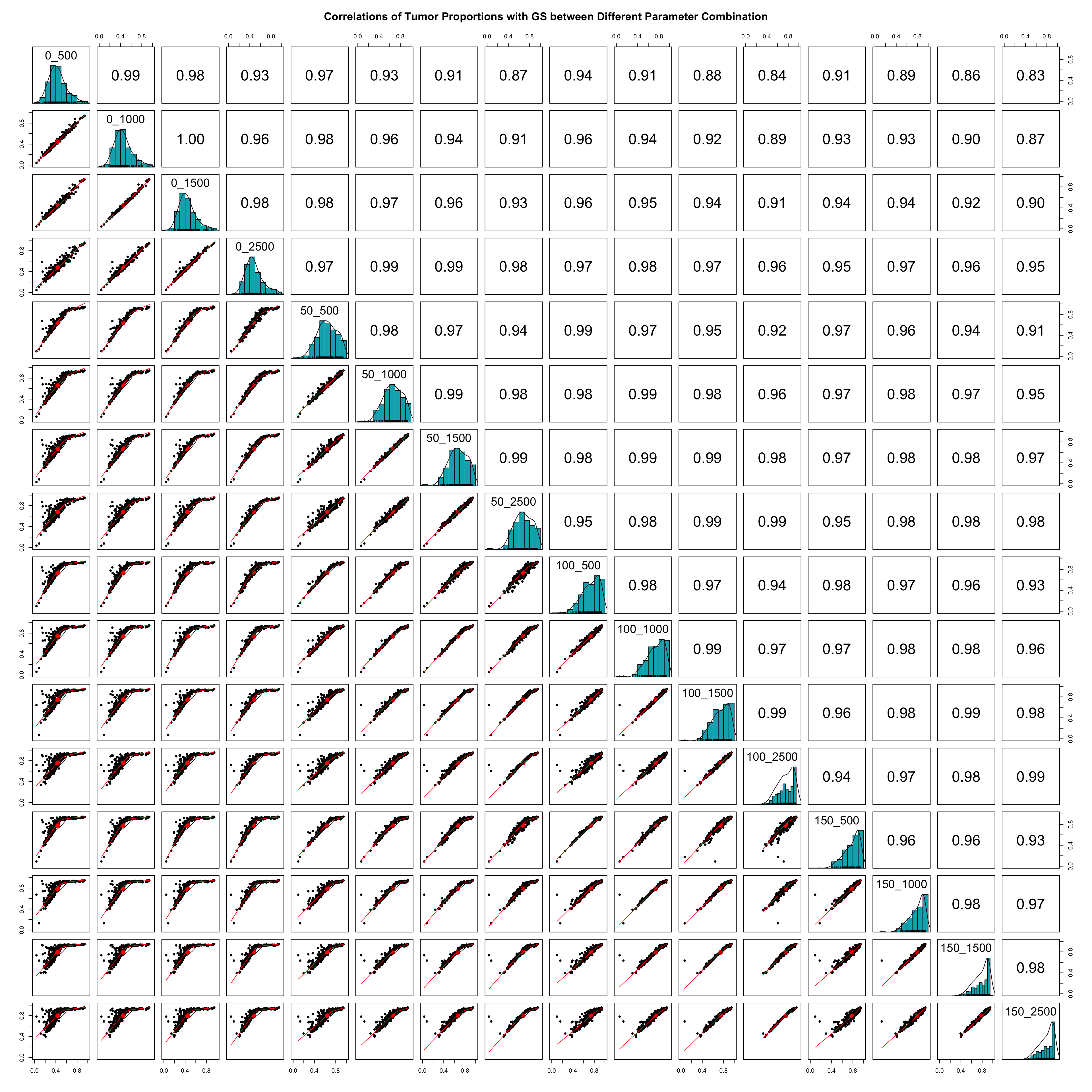
This step saves the deconvolution results (PiT) into a dataframe with columns named after the combination of the number of spike-ins and number of genes selected. Then one can calculate and plot the pairwise correlations of estimated tumor proportions across different parameter combinations as shown in the next slide.
pairs.panels(PiT_GS_PRAD,method ="spearman", # correlation methodhist.col ="#00AFBB",density =TRUE, # show density plotsellipses =TRUE, # show correlation ellipsesmain ='Correlations of Tumor Proportions with GS between Different Parameter Combination',xlim =c(0,1),ylim =c(0,1))
Print out the average pairwise correlation of tumor proportions across different parameter combinations.
We suggest selecting the optimal parameter combination that produces the highest average correlation of estimated tumor proportions.
Additionally, users are encouraged to evaluate the skewness of the PiT estimation distribution compared to a normal distribution centered around 0.5, as Significant skewness may indicate biased estimation.
Based on these criteria, spike-ins = 5 and number of selected genes = 1000 are identified as the optimal parameter combination. Using these parameters, we can obtain the corresponding tumor proportions.
Instead of selecting using the parameter combination with the highest correlation, one can also select the parameter combination that produces estimated tumor proportions that are most biologically meaningful.
Next,
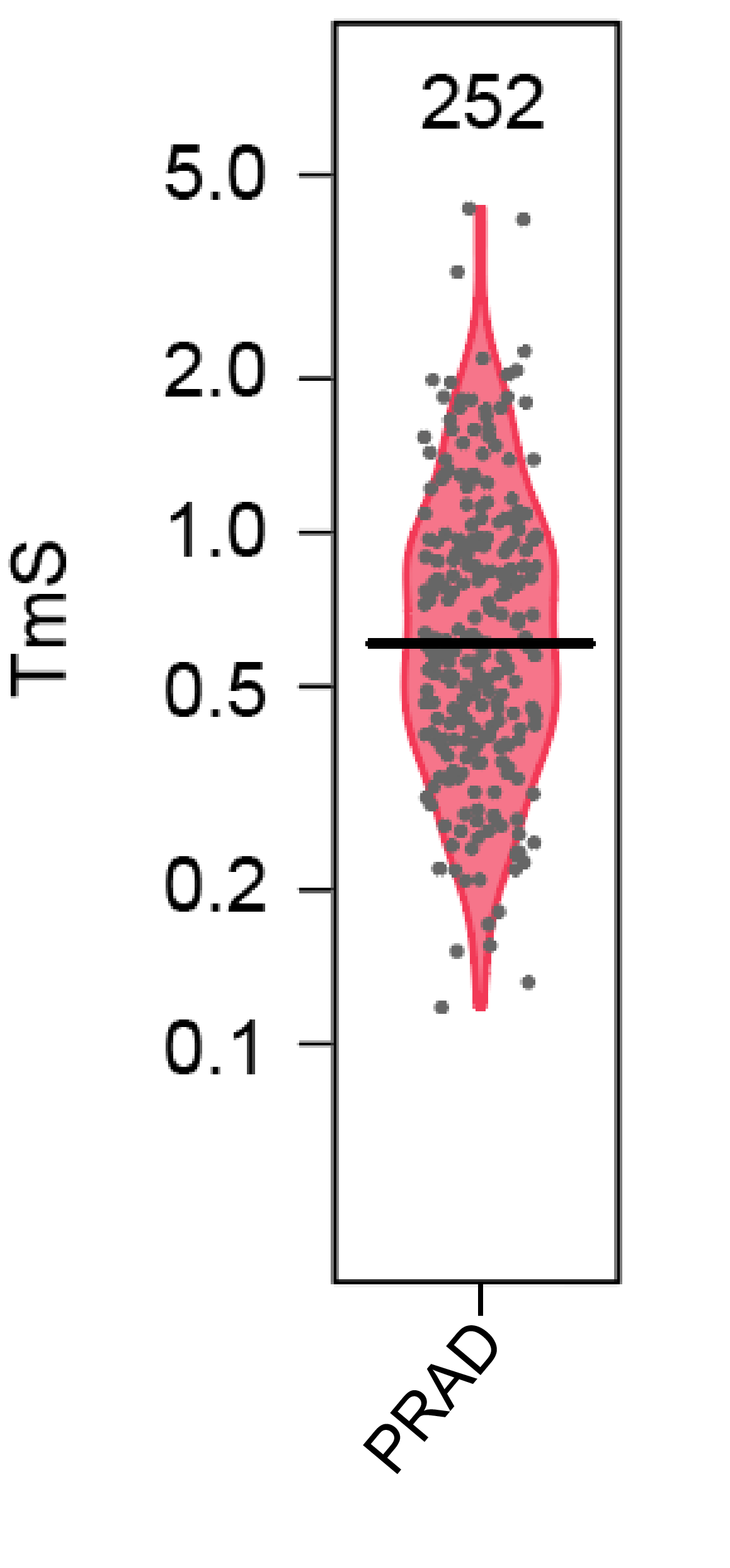
We will provide a simple TmS tutorial which uses The estimated tumor-specific proportions (PiT) genertated from DeMixT. For more details, visit https://wwylab.github.io/TmS/articles/TmS.html.
TmS Calcualtion
Tumor-specific total mRNA expression (TmS) from bulk sequencing data, taking into account tumor transcript proportion, purity and ploidy, which are estimable through transcriptomic/genomic deconvolution.
TmS analysis pipeline consists of the following steps:
Step 1: Estimate the proportion of total RNA expression (\(\pi\)) from tumor cells using RNAseq data.
Achieved by using DeMixT[1]
Step 2: Estiamte the proportion of tumor cells and total copies of haploid genomes, i.e., tumor purity (𝜌) and tumor ploidy (\(\psi\)), using matched DNAseq or SNP array data.
Step 3: Calculate TmS, the per cell haploid genome total RNA expression for tumor, using the estimated (\(\pi\)), (𝜌) and (\(\psi\)): \(TmS=[\pi (1-𝜌)2]/[(1-\pi)𝜌\psi]\).
Step 3: Calculate TmS using the estimated (\(\pi\)), (𝜌) and (\(\psi\)).
Consensus TmS estimation
For DNA-based deconvolution methods such as ASCAT and ABSOLUTE, there could be multiple tumor purity 𝜌 and ploidy \(\psi\) pairs that have similar likelihoods. Both ASCAT and ABSOLUTE can accurately estimate the product of purity 𝜌 and ploidy \(\psi\); however, they sometimes lack power to identify and separately. TmS is derived from the product of tumor ploidy and the odds of tumor purity. Hence, it is potentially more robust to ambiguity in the tumor purity and ploidy estimation, ensuring the robustness of the TmS calculation.
To calculate one final set of TmS values for a maximum number of samples, we use a consensus approach. We first calculate TmS values with tumor purity and ploidy estimates derived from both ABSOLUTE and ASCAT, and then fit a linear regression model on the log2-transformed \(TmS_{ASCAT}\) using the log2-transformed \(TmS_{ABSOLUTE}\) as a predictor variable. We remove samples with Cook’s distance ≥ 4/n and calculate the final
The agreement between the two methods in ploidy values was low in 20% of TCGA samples. However, a large portion of these samples showed consistency in the TmS values using either ASCAT and ABSOLUTE, reducing the number of filtered TCGA samples to ~5% (264 samples) [2]. This result supports the robustness of our consensus approach.
Input: Tumor-specific total mRNA proportions, tumor purities, tumor ploidies
Output: Consensus TmS
p: Tumor-specific total mRNA proportions estimated by DeMixT
[2] Cao, S. et al. Estimation of tumor cell total mRNA expression in 15 cancer types predicts disease progression. Nat Biotechnol (2022). https://doi.org/10.1038/s41587-022-01342-x.